Mapping zooplankton distribution with archived acoustic data
Digging up old acoustic data to study the distribution of krill, salps, and other creatures along the Antarctic Peninsula
ADCP Backscatter Visualization: Demo Video | Interactive Map (Javascript) | Interactive Map (Python via JupyterLite)
In this project, we re-analyzed archived data from an Acoustic Doppler Current Profiler (ADCP) to investigate the distribution of key macrozooplankton/micronekton, particularly Antarctic krill, in the Southern Ocean along the western Antarctic Peninsula. Krill are a key species for both predators and fisheries in this region, but our work suggests that climate change has resulted in increasingly long shortages of krill that are having dramatic impacts on the ecosystem.
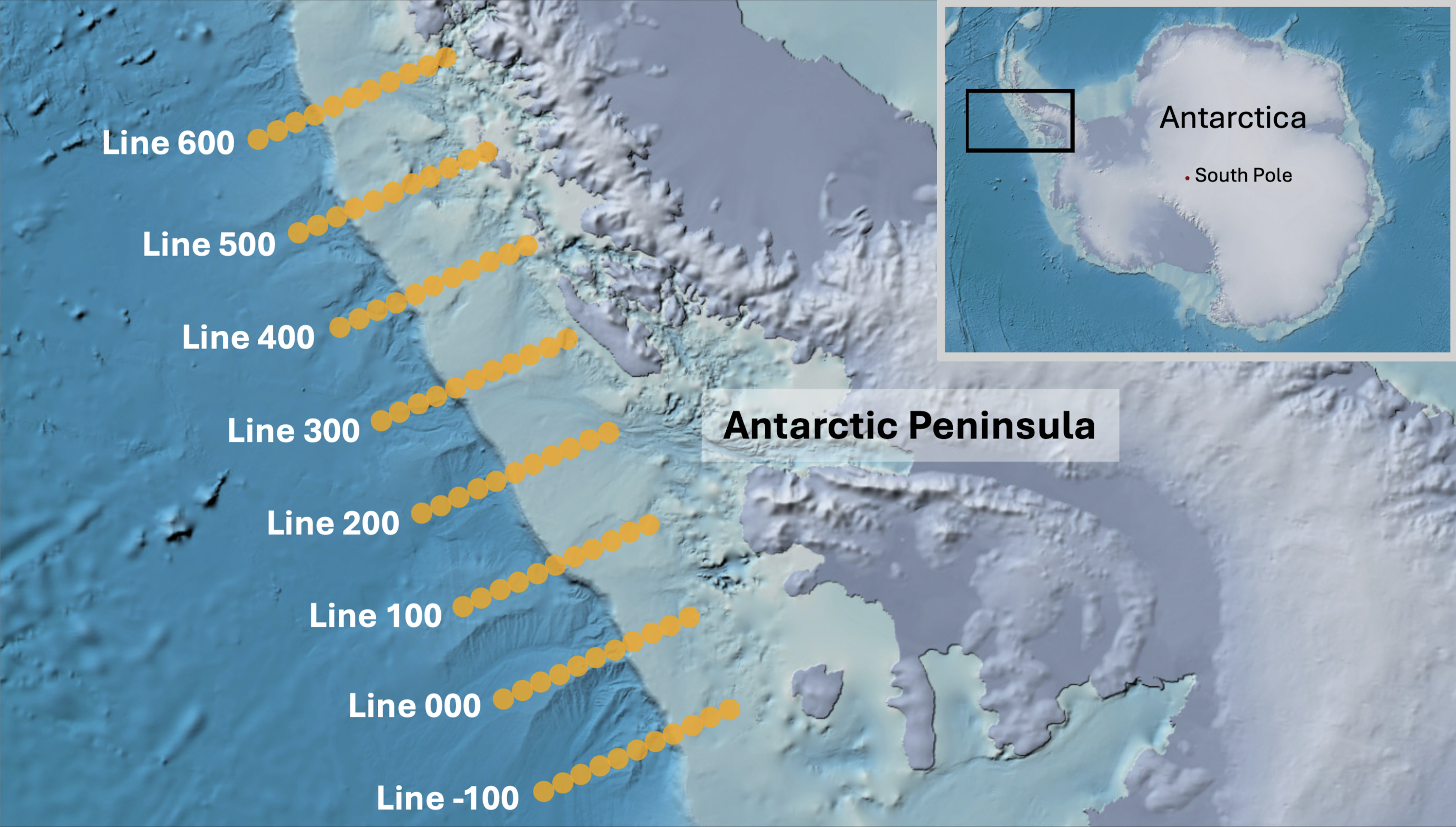
Every year, the Palmer Station Long-Term Ecological Research (LTER) project runs a research cruise in the Southern Ocean, tracing a sampling grid along the western Antarctic Peninsula.

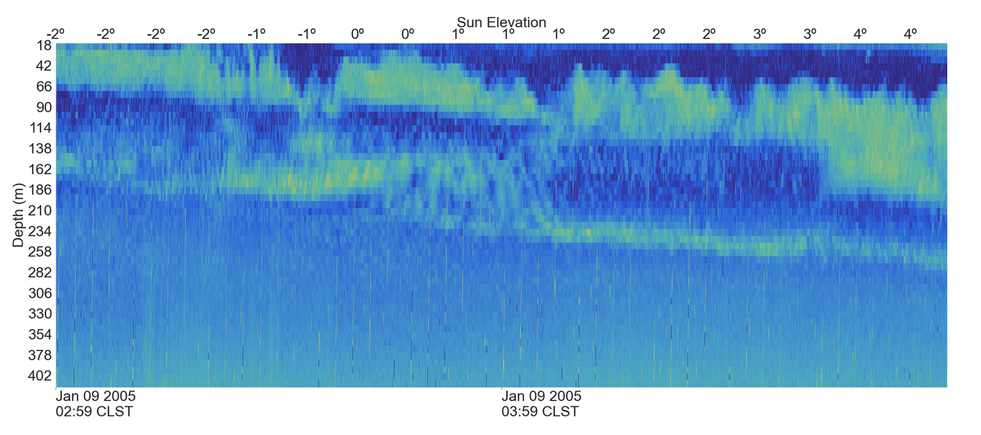
The vessel has a hull-mounted Acoustic Doppler Current Profiler (ADCP). An ADCP is an acoustic instrument that uses sonar to measure water velocity throughout the water column - it’s used to map oceanographic currents and water movement. The ADCP sends out pings of sound and listens for the returning echoes. It records two properties of the echoes: the echo frequency and the echo intensity (or loudness). Based on the echo intensity, we can estimate backscatter intensity - that is, the acoustic reflectivity of objects at a given depth in the water column. The backscatter intensity gives a sense of the presence and size/density of objects in the water below the ADCP - a dense school of krill will have a backscatter intensity (that is, high acoustic reflectivity), while a mostly empty water column will have a very low backscatter intensity (it’ll produce only a very quiet echo).

I reprocessed archived ADCP data from Palmer Station LTER cruises from 2005 through 2018 - a total of over 32 million sonar pings! - to examine the horizontal and vertical distribution of organisms in the water column. By combining this information with net tows (in which a net is towed to sample the organisms in the water column) performed by the Palmer Station LTER project, we could get a sense of both the horizontal and vertical distribution of biomass, as well as the identity of the organisms making up the big swarms we can see in the acoustic data. I mentored 3 students (Jon Michael Stroh, Nichole Zhang, and Leif Kelley) through Duke University Data Science’s undergraduate research program, and we built a GUI using Python’s ipyleaflet to allow us to visualize and walk through these data. We combined the ship’s track with several datasets: ADCP echo intensities, net tows, sun elevations, and temperature-depth profiles taken at stops along the cruise track. A JupyterLite version of the Python visualization can be run here, and I built a more browser-friendly version in JavaScript using Leaflet which can be viewed here. (JupyterLite doesn’t yet work reliably in all browsers.) There’s a demo/tutorial video here showing the Python version.
Data processing pipeline
The ADCP records data in a custom binary encoding unique to the manufacturer. Unfortunately for me, existing ADCP processing software focuses on creating spatially averaged estimates of water velocity and does not save the echo intensities, nor does it convert many of the other measurements tracked by the ADCP (such as temperature at the transducer)… so I had to use the manufacturer’s manual and write code to parse the binary myself. In the processing pipeline, I first convert from the ADCP’s raw binary data files to human-readable csvs.
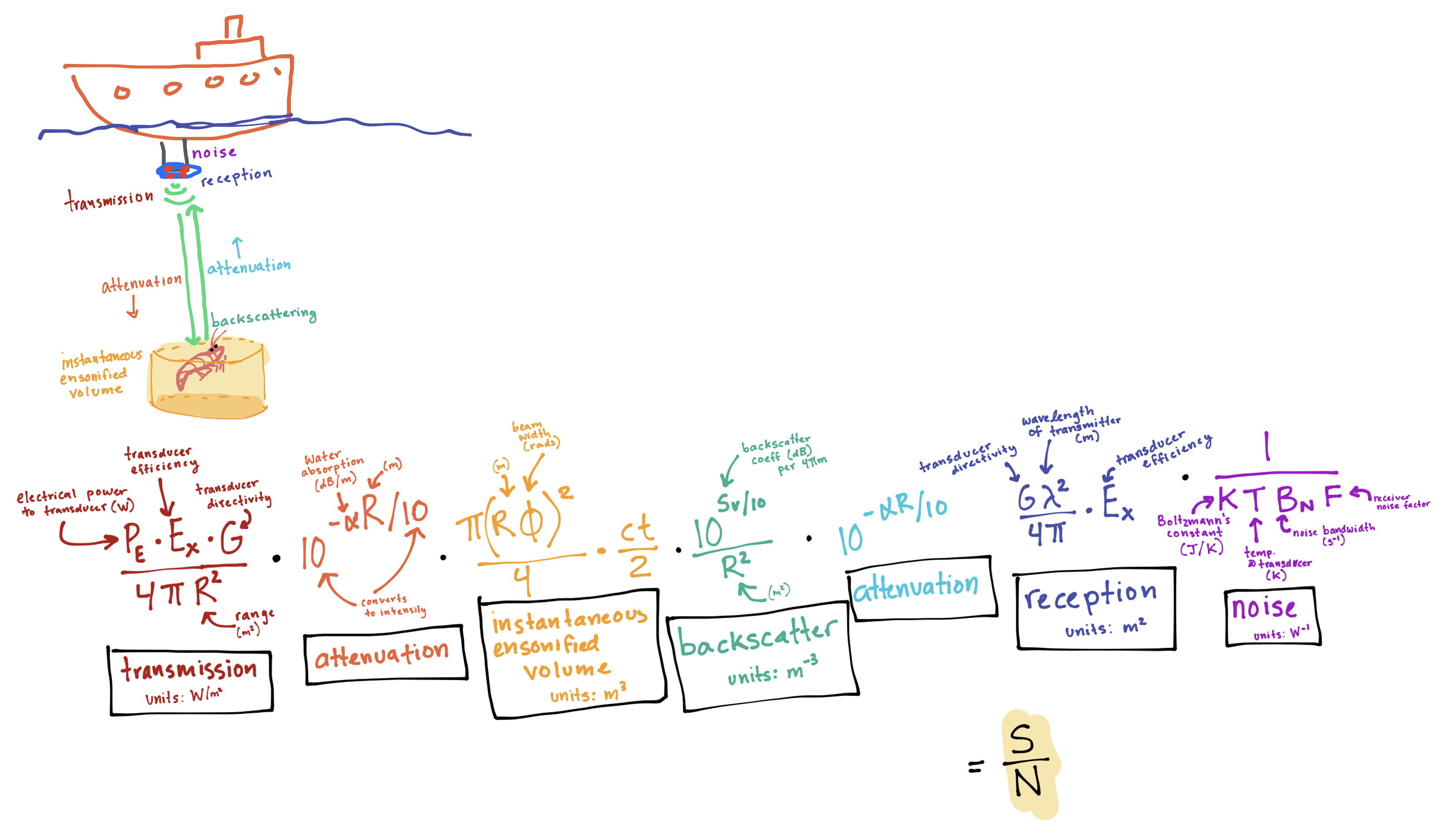
The ADCP records a relative value of the echo’s sound power as an 8-bit number representing the electrical signal induced in the transducer by the echo. Unfortunately again, the relationship between this value and the actual echo intensity in real-world units is non-linearly related to a host of variables including temperature at the transducer, water temperature, and water salinity, and it must then be corrected for depth. I then perform this conversion, using the sonar equation to calculate the approximate echo intensity in real-world dBs.
